New features in R

A look at the new features introduced in the 4.0 version of R

> Photo by Clint Patterson on Unsplash

Recently I had updated my RStudio client and with it came a new update to R. This is an exploration of some of the most interesting changes from R 4.0 to R 4.1.

Native Pipe Function

Due to the extreme popularity of the magrittr pipe (‘%>%’), R has developed its own native pipe (‘|>’).

library(tidyverse)
data("morley")
morley |>
        group_by(Expt) |>
        summarise(mean = mean(Speed, na.rm=TRUE))

# A tibble: 5 × 2
   Expt  mean
  <int> <dbl>
1     1  909 
2     2  856 
3     3  845 
4     4  820.
5     5  832.

From this example, it is apparent that the behaviour of the native pipe is the same as the magrittr pipe.

Some of the differences I have found is that the native pipe requires the brackets for functions, while the magrittr pipe will usually accept just the function name.

2 %>% sqrt()

[1] 1.414214

2 |> sqrt()

[1] 1.414214

2 %>% sqrt

[1] 1.414214

2 |> sqrt

Error: The pipe operator requires a function call as RHS

One disadvantage of the native pipe is that it doesn’t support the placeholder operator (.) which helps refer to the data in the function. This is a useful function of the magrittr pipe when the data isn’t the first argument in the function, such as the lm function.

morley %>% lm(Speed~Run, data = .)

Call:
lm(formula = Speed ~ Run, data = .)

Coefficients:
(Intercept)          Run  
   856.0947      -0.3519  

morley |> lm(Speed~Run, data = .)

Error in is.data.frame(data): object '.' not found

One advantage is there is no performance penalty as it acts the same as the function call. This is shown with the microbenchmark function, which shows not only the same level of performance as the regular call, but even the results themselves are shown as the function call.

library(microbenchmark)
microbenchmark(sqrt(3),
               4 |> sqrt(),
               5 %>% sqrt())

Unit: nanoseconds
         expr  min   lq mean median   uq   max neval
      sqrt(3)    0   50  146    100  100  6800   100
      sqrt(4)    0    0   42      0  100   300   100
 5 %>% sqrt() 2300 2400 2730   2400 2500 26100   100

So when should we use the native vs the magrittr pipe? Well, it looks like not all the functionality of the magrittr pipe is carried over, so it should still be continued to be used. The native pipe, however, provides a good performance boost, which makes it a better option for code written in functions and libraries. I think that the major application should be to increase the readability of library and function code.

Lambda Functions

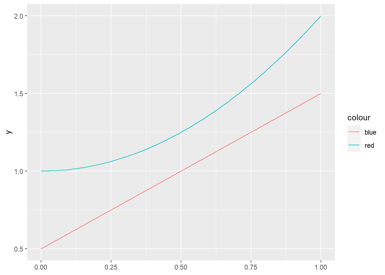
There has been a simplification in the creation of lambda functions. The notation is simplified, while the results are the same.

library(tidyverse)
x <- 0:10/10
y1 <- function(x) x + 0.5
y2 <- \(x) x^2 +1
g <- ggplot(data.frame(x=x)) +
        geom_function(fun = y1, aes(color = "blue")) +
        geom_function(fun = y2, aes(color = "red"))
g

Other minor changes

• The default has been changed for ‘stringsAsFactors = FALSE’. Previously, when using the data.frame() or the read.table() the default option would turn strings into factors. This was an annoying feature that would always create headaches.
• Introduction of an experimental implementation of hash tables. This development should be watched for people keen on program performance.
• c() can now combine factors to create a new factor. I am not familiar with the original behaviour, but this seems intuitive.