Code
library(tidyverse)
download.file("https://www.openml.org/data/download/41/dataset_41_glass.arff", "data.arff")
df <- farff::readARFF("data.arff")
I was recently reading my copy of “An Introduction to Statistical Learning” (my Amazon affiliate link) and got the chapter about the different tree based methods. I am pretty familiar with Random Forest, but a few of the other methods are new to me. Let’s explore these different techniques.
For these examples, I will explore the glass dataset from the openml site. This dataset has 9 different features used to predict the type of glass. The dataset has 214 observations.
The dataset is downloaded with the following code. This requires the farff package to open the arff files used on the openml site.
library(tidyverse)
download.file("https://www.openml.org/data/download/41/dataset_41_glass.arff", "data.arff")
df <- farff::readARFF("data.arff")From there, we can start to explore the dataset and set up a train and testing split for the data.
df %>% str()'data.frame': 214 obs. of 10 variables:
$ RI : num 1.52 1.52 1.52 1.51 1.53 ...
$ Na : num 12.8 12.2 13.2 14.4 12.3 ...
$ Mg : num 3.5 3.52 3.48 1.74 0 2.85 3.65 2.84 0 3.9 ...
$ Al : num 1.12 1.35 1.41 1.54 1 1.44 0.65 1.28 2.68 1.3 ...
$ Si : num 73 72.9 72.6 74.5 70.2 ...
$ K : num 0.64 0.57 0.59 0 0.12 0.57 0.06 0.55 0.08 0.55 ...
$ Ca : num 8.77 8.53 8.43 7.59 16.19 ...
$ Ba : num 0 0 0 0 0 0.11 0 0 0.61 0 ...
$ Fe : num 0 0 0 0 0.24 0.22 0 0 0.05 0.28 ...
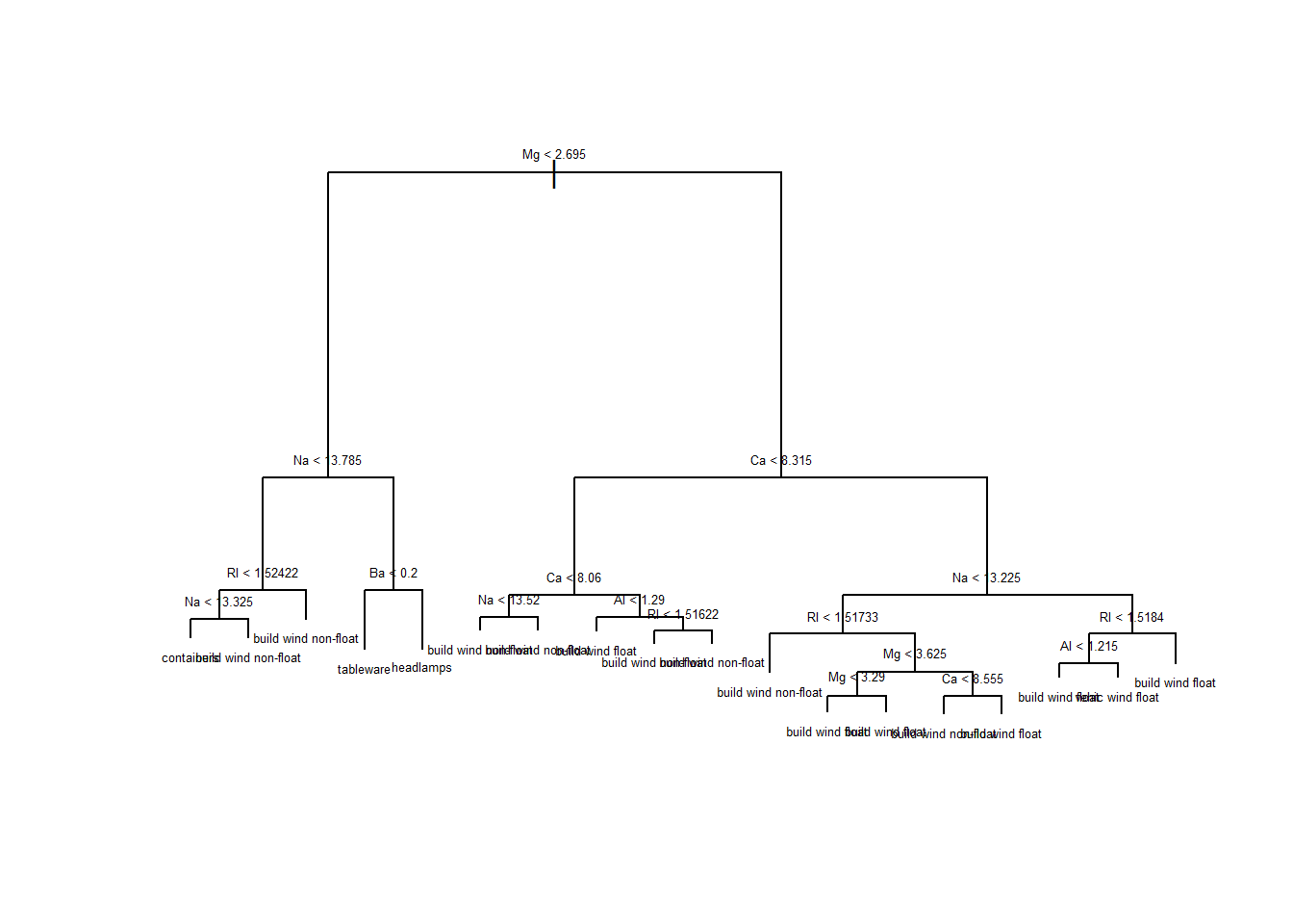
$ Type: Factor w/ 7 levels "build wind float",..: 1 3 1 6 2 2 3 1 7 2 ...The most basic model is the decision tree. In this model, all classes are stored in a container at the root of the tree. The root is split by certain feature values into two smaller containers. These smaller containers are called leafs. After these initial two leafs, we perform an additional split resulting in 4 new leafs. At this point, there should be some better sorting on the response value in the new leafs. Splitting and creating new leafs is continued until the desire results are obtained.
The main disadvantage of decision trees is that they are very prone to over fitting. It is pretty easy to imagine a tree that has split so many times that each leaf now represents a single observation. This tree would have 100% accuracy on the training set, but would not perform well on a test set. We prevent over fitting by cutting off or pruning the number of leafs to a certain value.
For our example, the decision tree is created with the tree package. It is pretty simple to use, you just supply it with the function and the data.
mdltree <- tree::tree(Type ~., data = traindf)A tree visualization is easily created with the print command. With an extra line, we can add the text that shows where each leaf is split. It does get difficult to understand the splits when getting to the lower level leafs.
We can now test the decision tree’s performance on the test data. Since the response is a factor, the resulting prediction is a matrix with a probability assigned to each response for every observation. We can summarize the mostly likely response with the max.col function.
[1] 0.5From this prediction, we can see that the decision tree didn’t provide a high level of accuracy (50% Accuracy). For a higher level of accuracy, let’s explore some additional methods.
Bootstrapping is a useful technique when we have a limited number of observations. Ordinarily, we take each training observation out of a bag and train our model with it. In bootstrapping, after we train our model with an observation, we put the observation back in the bag, allowing repeated selection. The repeated selection creates a smoother distribution of observations.
Bagging takes this process one step further. We take multiple models from bootstrapped training data and average their values. Each bootstrapped model is unique because the training observations are randomly selected.
Bagging can be performed with the randomForest function. By default, the function creates trees from a subset of features, but we can create bagged trees by using all features. The default behaviour for a random forest is to take the majority vote for constructed trees or average their prediction.
library(randomForest)
mdlbag <- randomForest(Type ~., data = droplevels(traindf), mtry = ncol(df)-1, n.trees = 500)
bagpreds <- predict(mdlbag, newdata = testdf)
Accbag <- mean(bagpreds == testdf$Type)
Accbag
[1] 0.6666667A random forest is an ensemble model, meaning the prediction is created by combining multiple models together. It is very similar to the previous example with Bagging. The main difference is that the Random Forest selects a random set of features when creating each tree.
The rationale for a random feature selection is to create more unique trees. If there is a strong feature in bagging, then most of the trees will use it to create their first split. This creates trees that appear very similar.
mdlforest <- randomForest(Type ~., data = droplevels(traindf), n.trees = 500)
rfpreds <- predict(mdlforest, newdata = testdf)
Accrf <- mean(rfpreds == testdf$Type)
Accrf
[1] 0.6666667Boosting is another multiple use technique, much like bagging. Instead of effecting the train data to create different trees, boosting builds trees in sequential order with the default training set. Rather than fitting trees to the response, trees are fit to their residuals. Each tree then learns slowly with the residuals from the previous tree.
For this model, we will to use two libraries, caret and gbm. The gbm package is the package that provides the actual model, but a warning is displayed when using the gbm function. To get around the issue, we can use the caret package with the train function. This function can accept many different models and will automatically go through tuning parameters.
Bayesian Additive Regression Trees (BART) are similar to the previously mentioned models, creating trees with some random elements that model the signal not captured in previous trees.
In the first iteration of the model, all trees are initialized to the same root node. After other iteration updates each of the kth trees one at a time. During the bth iteration, we subtract the predicted values from each response to produce a partial residual. i represents each iteration.
\[ r_i = y_i - \Sigma_{k'<k}f^b_{k'}(x_i) - \Sigma_{k'>k}f^{b-1}_{k'}(x_i) \] Rather than fitting a new tree to this residual, BART randomly chooses a tree from the previous iteration (\(f^{b-1}_k\)), favouring trees that improve fit.
Unfortunately, I have not been able to get any BART model to work for this multi-class classification example. The bartMachine package doesn’t have an implementation, and the BART package’s implementation doesn’t seem to work for me. All the values for me were returning NA. There is also very little resources on the BART package to troubleshoot.
The decision tree as an easy-to-understand model, but they are prone to over fitting data. Pruning is required to reduce this, but will also reduce accuracy(50% Accuracy for this example).
Ensemble models are then introduced with Bagging which averages a bunch of trees created by a selection of different observations. This does increase our accuracy(66.67%). This is very similar to the Random Forest model, but instead we increase the random element to include the features selected (66.67%).
The final models create trees that build of previously generated trees with the boosting and the Bayesian Additive Regression Tree. Unfortunately, there are no results for the BART model, but boosting does produce good results (69.05%).
So there is no clear answer which model is the best, they follow pretty similar methods and produce similar results. I would recommend training them all and finding which performs best on your data.